My Learning Archive

Explore key concepts in electronics with visual summaries


Small Signal Analysis of BJT

This section might summarizes the small signal analysis of a Bipolar Junction Transistor (BJT) with H-parameter model, Check this book for more knowledge and equations.


This is the circuit diagram of Common Collector: Small Signal Analysis of BJT


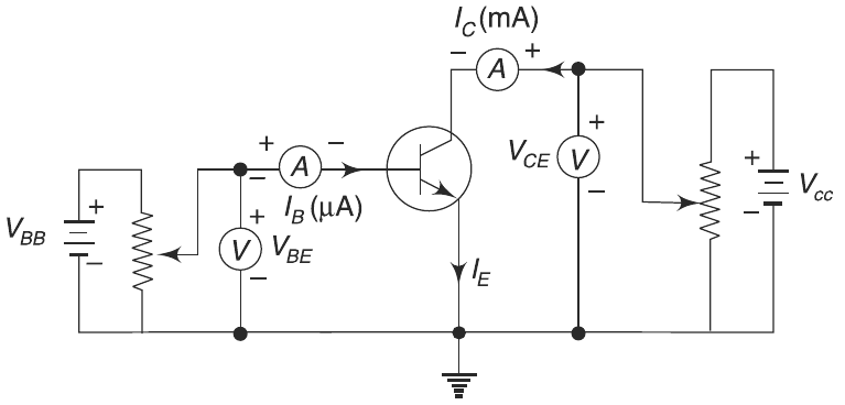
This is the circuit diagram of Common Emmiter: Small Signal Analysis of BJT
So the H-Parameter model and its Gain and Impedence are :
Current Gain \(A_i\) = - \(\frac{I_c}{I_b}\)
Voltage Gain \(A_v\) = - \(\frac{A_i * R_l}{Z_i}\)
Input Impedence \(Z_i\) = \(H_ie\) - \(\frac{H_re*H_fe*R_l}{1+H_oe*R_l}\)
Output Impedence \(Z_o\) = \(R_l\)


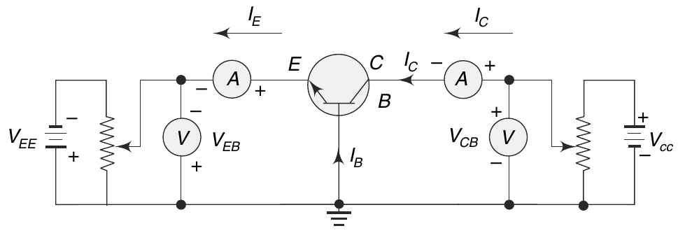
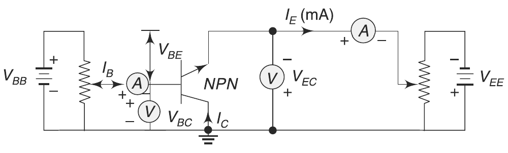
This is the circuit diagram of Common Base: Small Signal Analysis of BJT

Characteristic Model of MOSFET

Characteristic model of Metal-Oxide-Semiconductor Field-Effect Transistor (MOSFET), \[ h_{ib} = \frac{\partial V_{EB}}{\partial I_E} \]

Characteristic Model of MOSFET

Basics of Control System

Lets consider a example :

Here we know a mechanical system that is damped (bx) and Spring (k) with distance or displacement (x) with Force (F).
The modeling equation of this system is
\[ M \frac{d^2x}{dt^2} + b \frac{dx}{dt} + kx = F \]
Taking the Laplace transform \[ Ms^2X(s) + bsX(s) + kX(s) = F(s) \]
Now the transfer function between the displacement \(X(s)\) and the input \(F(s)\):
\[ \frac{X(s)}{F(s)} = \frac{1}{Ms^2 + bs + k} \]

GHDL + GTKWave

24/04/2026


Recently i learned Vhdl and found Ghdl with GTKWave and heres the flow
(this is more of a entry then a proper way to learn, if in case you want to learn try finding a tutorial and follow it with different example. For this i found and gate example and extend it to 4-bit BCD to Excess-3),

(Main file)

1) Import library and define module
2) Create entity for this blackbox and assign ports for in and out and end the entity (entity name should be your file name).


3) Add a architecture with whatever name you like (here "rtl_of_blackbox" is used)
and begin assigning logic to "out" port/s and end it.


(Test file)

1) Now for test file, add library, create entity (same file name) and end the entity; 2) The port for our blackbox is already assigned in main file so we will assign those in component under architecture.
Here, "Test2" is main file and "testfor2" is our test file (All these .vhdl files are compiled into folder);


3) Here i dont have any wires so i allotted all my ports as signal and the output of port as standard logic;
4) Now map those ports and write testcases. BCD to Excess-3 of 4 port in and 4 port out suppose to have 24 possibilities and i only used 4 of them;


5) Now end the process and architecture;


Outputs


$ ghdl -a main_file*.vhdl $ ghdl -a test_file*.vhdl $ ghdl -r main_file* $ ghdl -r test_file*
testfor2.vhdl:51:6:@4ns:(assertion error): End of Test
$ ghdl -r test_file* --vcd=B2E3.vcd
testfor2.vhdl:51:6:@4ns:(assertion error): End of Test
$ gtkwave B2E3.vcd
The files are compiled into a folders with its file names so the way you visualize using gtkwave is by re-compiling that test folder into a *.vcd* file which can be opened with gtkview directly.
The only issue with HDL is we have to make a test_case which makes the whole "Fool Around and Find Out" concept into desired input and output.